Hydrogen Spectrum : Lines, Series and Everything

The hydrogen spectrum is the electromagnetic radiation emitted by the electron of excited hydrogen when it returns to a normal state. The energy radiated corresponds to the wavelength of the hydrogen spectrum.

Before discussing the hydrogen spectrum we shall briefly discussed the spectra in general.

Incandescent solids and liquids, when white hot, emit continuous spectrum (e.g., the solar spectrum). Gases and vapours give line spectra and band spectra (in addition to the continuous region). The line spectra belong to the atoms and the band spectra to the molecules, whereas the continuous spectra can occur in the case of atoms as well as molecules.

Line and Band Spectra

The line spectra consists of discrete lines or complexes of lines. There exist regular sequences of lines within the line spectra. These sequences may be grouped together into series. In each series, the distance between successive lines decreases according to definite laws as we proceed towards the violet end of the spectra and the lines accumulate at a series limit. The intensity of the lines in a series decreases regularly towards the series limit, as is the rule, from the beginning of the series or from a definite point later.

A band spectra is obtained if the dispersion is small. It consists of shaded bands, one edge of which is sharp, but the intensity of light falls off at the other edge. The band spectra resolve under higher dispersion into a large number of neighbouring lines. The lines of a band spectrum accumulate at the head of the band, but do not become infinitely dense there as in the case of lines at the series limit in the line spectrum. The heads of the bands are situated partly towards the violet and partly towards the red.

Shaded Bands to Fraunhofer Lines

The line spectra and band spectra occur both during absorption as well as emission. Indeed it was the absorption spectra in the form of Fraunhofer lines (the dark lines observed in the solar spectrum are known as Fraunhofer lines) which primarily played the determining role in the historical development of the spectrum analysis.

The simplest line spectrum is that given by the simplest atom-hydrogen. It has a series of lines whose intensity and separation decrease in a perfectly regular manner towards the shorter wavelengths. The spectra of all other elements similarly consists of such series of lines, which however are not always so easily recognisable due to much overlapping.

Four of the most prominent lines of the hydrogen spectrum were first measured by Fraunhofer as the absorption lines of the solar spectrum. These lines were called the C, F, f, h lines and are now referred to as H_α, H_β, Н_γ and H_δ.

Equations for Balmer series

Balmer was the first to formulate a law of the entire hydrogen series in 1885. He showed that within experimental error, the wavelengths of the then known spectral lines in the hydrogen spectrum could be expressed by the formula,

$.\;\;\;\;\;\;\;\;\;\;\;\;\;\;\;\lambda=a\frac{n_2^2}{n_2^2-n_1^2}$ ……………….. (1)

where a=3645.6, n₁=2 and n₂=3,4,5,6…. for the first, second, third…… members of the series, the first four values of n₂ being those corresponding to H_α, H_β, Н_γ, H_δ . The Balmer’s formula, eqn. (1), can be re-written in slightly different manner by inverting both sides of the equation.

$.\;\;\;\;\;\;\;\;\;\;\;\;\;\;\;\;\;\;\frac1\lambda=\frac1a-\frac{n_1^2}{{an_2}^2}$

Putting $\frac1\lambda=\overline{\nu_n}$ the wave number (number of waves per meter) and $\frac{n_1^2}a=R$ , this gives

$.\;\;\;\;\;\;\;\;\;\;\;\;\;\;\;\;\;\;\;\overline{\nu_n}\;=R\left[\frac1{n_1^2}-\frac1{n_2^2}\right]$ …………….. (2)

where R is known as Rydberg constant. This equation represents what is known as the hydrogen series formula. It gives the wave number $\overline{\nu_n}$ as the difference of two terms, the first $\frac R{n_1^2}$ being the constant term (as n₁ has a constant value 2) which at the same time gives the series limit (n₂= ∞) and the second term $\frac R{n_2^2}$ being a variable term.

This representation of $\overline{\nu_n}$ as the difference of two terms corresponds to the view of the wave number as the difference of level between two energy steps. The terms therefore give us the energy of the atom in its initial and final states.

Also Read : Photo Electric Effect : Definition, Types and Everything

Rydberg-Ritz Combination Principle

According to this principle, within certain limitations, the difference between any two terms of an atom gives the wave number of a spectral line of the atom. For instance if the term differences, A – B and C – D represent two lines then new lines with wave number A – C, B – D, A – D and B – C would result by combining the terms (A, C), (B, D), (A, D) and (B, C) respectively.

The truth of this principle of combination was first tested by employing the hydrogen spectrum. Balmer suspected that the number n₁ in his formula might also take the value 3. In other words he suspected the existence of the spectral lines with wave numbers

$.\;\;\;\;\;\;\;\;\;\;\;\;\overline{\nu_n}\;=R\left[\frac1{3^2}-\frac1{4^2}\right],\;\;\;\;\;\;\overline{\nu_n}\;=R\left[\frac1{3^2}-\frac1{5^2}\right],\;etc.$

The existence of these lines was demanded by Ritz since the first of these lines may be obtained by forming the difference of the wave numbers of H_β and H_α while the second may be obtained by forming the difference of the wave numbers of Н_γ and H_α, [the wave numbers of H_α, H_β, and H_δ are respectively given by $R\left[\frac1{2^2}-\frac1{3^2}\right],\;R\left[\frac1{2^2}-\frac1{4^2}\right],\;\;and\;R\left[\frac1{2^2}-\frac1{5^2}\right]$ and so on. These lines were later actually shown to exist in the infrared region by Paschen. Later on more lines were found; all these could be explained by giving running values to n₁ and n₂ in the Balmer’s formula

$.\;\;\;\;\;\;\;\;\;\;\;\;\;\;\;\;\;\;\;\overline{\nu_n}\;=R\left[\frac1{n_1^2}-\frac1{n_2^2}\right]$

Equations for different serieses-

Giving n₁ the values from 1 to 5 the following formulae are obtained :

Lyman series: $\overline{\nu_n}\;=R\left[\frac1{1^2}-\frac1{n_2^2}\right]$ , n₂=2,3,4,….. ……….(3)

Balmer series: $\overline{\nu_n}\;=R\left[\frac1{2^2}-\frac1{n_2^2}\right]$ , n₂=3,4,5,….. ……….(4)

Paschen series: $\overline{\nu_n}\;=R\left[\frac1{3^2}-\frac1{n_2^2}\right]$ , n₂=4,5,6,….. ……….(5)

Brackett series: $\overline{\nu_n}\;=R\left[\frac1{4^2}-\frac1{n_2^2}\right]$ , n₂=5,6,7,…… ……….(6)

Pfund series: $\overline{\nu_n}\;=R\left[\frac1{5^2}-\frac1{n_2^2}\right]$ , n₂=6,7,8,….. ………..(7)

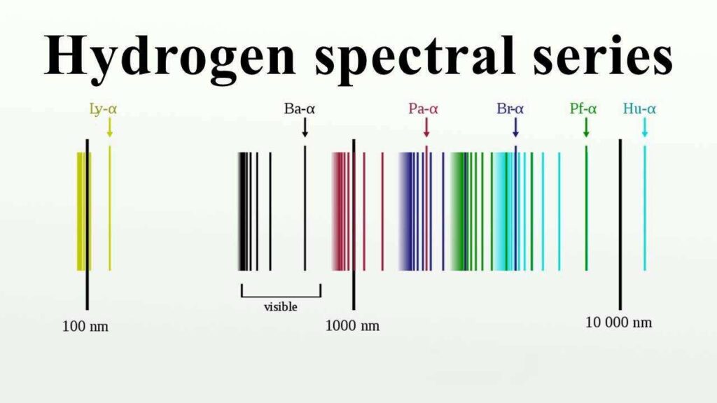
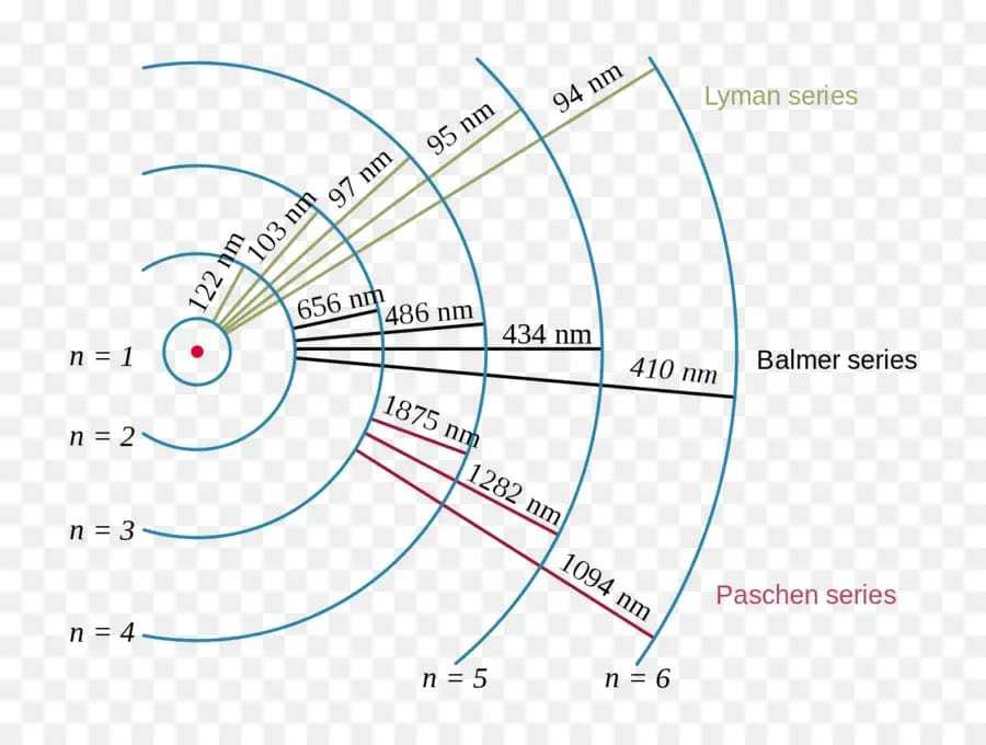
The first series, eqn. (3), was discovered by Lyman in the extreme ultra-violet region, the third series, eqn. (5), by Paschen as mentioned above and the fourth and fifth, eqns. (6) and (7), have been discovered when they were predicted by Brackett and Pfund respectively. The various series are shown in Fig., on a wavelength scale.

Hydrogen Spectrum (The various series of hydrogen atom)

According to the Balmer’s formula, eqn. (2), the wave number of any line of the hydrogen spectrum is given by the difference between two members of the series T(n) = R / (n²) having different values of n. The members are referred to as terms. The lines of other elements can similarly be predicted as difference between two terms. Therefore, the formula for the wave number of a line can be written as

$.\;\;\;\;\;\;\;\;\;\;\;\;\;\;\;\;\overline{\nu\;}=T_1-T_2$ …………………. (8)

The term T, however, usually has a somewhat more complicated form than that for the hydrogen atom.

The Balmer’s formula, eqn. (2), is not only a sufficient but also a necessary condition for the lines of hydrogen spectrum. In other words, not only all the series of lines indicated by this formula are actually observed in the case of hydrogen, but also no other lines belong to hydrogen atom except those contained in this formula.

Also Read : Einstein’s Theory of Relativity Explained : Space, Time, and Gravity

Pickering Series

Pickering in 1897 discovered a new series of lines in the spectrum of a star (named ξ-Puppis) whose wavelengths are closely related to the Balmer series of hydrogen spectrum. Rydberg showed that the new series could be represented by Balmer’s formula, eqn. (2), by allowing both integral and half integral values to n₂, i.e.,

$\overline{\nu_n}\;=R\left[\frac1{2^2}-\frac1{n_2^2}\right]$ , where n₂ = 2.5, 3, 3.5, 4, 4.5 …………… (9)

This gave very good consent between the calculated and experimental values of wavelengths. The Pickering series was therefore held responsible to some form of hydrogen found only in stars. However this series of lines has now been shown to arise from ionised helium (He⁺) and not from H, as a result of the experimental study of Evan, Fowler and Paschen. This series of ionised helium was explained by Bohr by extending his theory of hydrogen atom, as we shall see later.

We thus find that our assertion that the simple and integral character of the spectral laws expressed in Balmer’s formula represents a necessary and sufficient condition for emission by hydrogen is confirmed.

Bohr’s theory of hydrogen spectrum

Bohr in 1913 formulated a theory with the help of which he gave a satisfactory explanation of the Balmer, Lyman and Paschen series of hydrogen spectrum and the Pickering series of ionised helium. His theory is based on the principle of the quantum theory of radiation as enunciated by Planck and Einstein. He followed Rutherford and assumed that an atom consists of a positively charged nucleus surrounded by a cluster of electrons. The nucleus carries a positive charge equal to Ze where Z is the atomic number (or the number of electrons necessary to make the atom neutral) and e is the charge on the electron. In the case of hydrogen, he concluded, following Rutherford, that it consisted of a proton of charge +e = E in the nucleus and an electron of charge -e. He made the following assumptions in formulating his theory.

1. Bohr’s first postulate

According to Bohr’s, the electron rotates around the nucleus in circular orbits under the influence of a coulombian field of force. Since the mass of an electron had been shown to be much smaller as compare to a proton, he assumed at first that the nucleus is practically at rest. The force of attraction between the electron and the nucleus is-

$.\;\;\;\;\;\;\;\;\;\;F\;=\frac{eE}{4\pi\varepsilon_o\mathrm a^2}\;=\;\frac{Ze^2}{4\pi\varepsilon_oa^2}$ ………(10)

where ‘a’ is the distance between the electron and the nucleus (see the given figure). For hydrogen Z=1 for helium Z=2.

This coulomb’s force of attraction provides the required centripetal force mv²/a (where m is the mass of the electron and v is its velocity in the orbit) that is needed to keep the electron moving in a circular orbit of radius a. Therefore the condition for stable orbit is

$.\;\;\;\;\;\;\;\;\;\;\frac{Ze^2}{4\pi\varepsilon_oa^2}\;=\;\frac{mv^2}a$ …………….(11)

The velocity of the electron in its orbit is therefore given by

$.\;\;\;\;\;\;\;\;\;\;\;\;\;v^2\;=\;\frac{Ze^2}{4\pi\varepsilon_om\mathrm a}$ …………..(12)

Then the kinetic energy of the rotating electron is

$K.E.\;=\;\frac12mv^2\;=\;\frac12\frac{Ze^2}{4\pi\varepsilon_oa}\;=\;T$ ……….(13)

Assuming that the potential energy of the system (consisting of an electron and the nucleus) is zero when the electron is at an infinite distance the nucleus, the potential energy at a distance a from the nucleus is $\frac{Ze}{4\pi\varepsilon_oa}$ per unit positive charge. Hence, the potential energy of the electron at a distance ‘a’ from the nucleus is –

$.\;\;\;\;\;\;\;\;\;\;\;\;\;\;\;\;\;\;\;P.E.\;=\;-\frac{eZe}{4\pi\varepsilon_oa}\;\;\;\;\;\;\;\;\;\\;\;\;\;\;\;\;\;\;\;\;\;\;\;\;\;\;\;\;\;\;\;\;\;\;\;\;\;\;\;=\;-\frac{Ze^2}{4\pi\varepsilon_oa}=V\;=\;-2T$ …………(14)

Total energy-

The total energy W, being the sum of the kinetic energy and the potential energy of the electron, therefore-

$W\;=\;T+V\;=\;T-2T\;=-T\\;\;\;\;\;\;\;\;\;\;\;\;\;\;\;\;\;\;\;\;\;\;\;\;=\;-\frac{Ze^2}{8\pi\varepsilon_oa}$ …………(15)

This shows that the total energy of the electron in any closed orbit is negative. As we are concerned here only with the differences of energy the negative sign causes no difficulty whatsoever.

The above analysis is not by the electromagnetic theory which predicts that an accelerated charge would radiate energy in the form of electromagnetic waves. As an electron moving in a circular orbit would be continuously accelerated it must continuously lose energy, thereby spiraling inward as a decreases until it is swallowed up by the nucleus.

(See fig.)

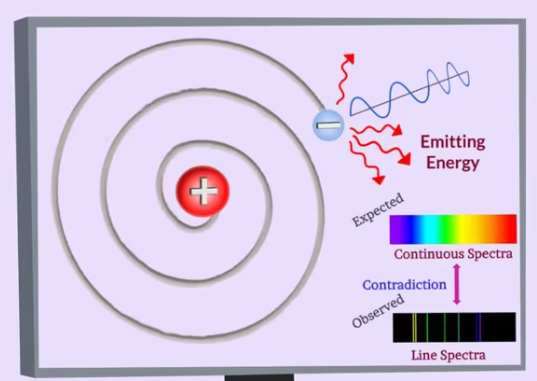
Bohr's first postulate (Hydrogen Spectrum)

The conventional physics therefore completely fails to account for the existence of stable atoms with electrons remaining at a distance from the nucleus.

Also Read : Understanding Secularism : Meaning, Importance and Impact on Society

2. Bohr’s second postulate

To maintain the stability of the electron into the nucleus, Bohr predicted the quantum hypothesis. He explained that the electron can move in only certain discrete non-radiating orbits, called stationary orbits. For which the angular momentum of the moving electron is an integral multiple of h /2π when h is the Planck’s constant.

$.\;\;\;\;\;\;\;\;\;\;\;\;\;\;\;\;\;\;\;\;\;\;\;\;\;\;\;I\omega\;=\frac{\;nh}{2\pi}$ ……………..(16)

where ‘I’ is stand for the moment of inertia of the electron about the nucleus, ω is its angular velocity and n is 1, 2, 3, … and is known as the principal quantum number. The angular momentum is thus said to be quantised. As I = ma² the above relation can also be written as

$.\;\;\;\;\;\;\;\;\;\;\;\;\;\;\;\;\;\;\;\;\;\;\;\;\;\;\;ma^2\omega\;=\frac{\;nh}{2\pi}$ ………………(17)

The kinetic energy of the electron is-

$.\;\;\;\;\;\;\;\;\;\;\;\;\;\;\;\;\;\;\;\;\;\;\;\;\;\;T=\frac12mv^2=\frac12m\left(a\omega\right)^2\\;\;\;\;\;\;\;\;\;\;\;\;\;\;\;\;\;\;\;\;\;\;\;\;\;\;\;\;\;\;\;\;\;\;=\frac12ma^2\omega^2$ …………….(18)

From eqn. (12), $v^2=a^2\omega^2=\frac{Ze^2}{4\pi\varepsilon_oma}$

$\therefore\;\;\;\;\;\;\;\;\;\;\;\;\;\;\;a^3\omega^2=\frac{Ze^2}{4\pi\varepsilon_om}$ ………….(19)

From eqn.(17), $\;a^2\omega=\frac{nh}{2\pi m}$ ………….(20)

Dividing eqn(19) by eqn(20) we get,

$.\;\;\;\;\;\;\;\;\;\;\;\;\;\;\;\;\;\;\;a\omega=\frac{Ze^2}{2\varepsilon_onh}$ ………….(21)

Substituting the value of aω in eqn.(18) we get,

$.\;\;\;\;\;\;\;\;\;\;\;\;T=\frac12m\left(\frac{Ze^2}{2\varepsilon_onh}\right)^2\\;\;\;\;\;\;\;\;\;\;\;\;\;\;\;\;\;\;=\frac{me^4Z^2}{8\varepsilon_o^2n^2h^2}=-W$ …………..(22)

Total energy-

$W=-\frac{me^4Z^2}{8\varepsilon_o^2n^2h^2}$ …………(23)

$or,\;\;W=\frac{RchZ^2}{n^2},\;\;\;where\;\;\;\;\;R=\frac{me^4}{8\varepsilon_o^2ch^3}$ is the Rydberg constant and is equal to 1.09678 x 10⁷ /m

In C.G.S. units $W=-\frac{2\pi^2me^4Z^2}{n^2h^2}$

The total energy of the electron is thus quantised in that it can take only discrete values determined by the integral values of the quantum number n. The energy content W has the algebraically smallest value in the first (innermost) orbit. If we call it W₁,then, for the second and third orbits respectively, we have

$.\;\;\;\;\;\;\;\;\;\;\;\;\;\;\;\;W_2=\frac14W_1\;\;\;and\;\;\;W_3=\frac19W_1$

These amounts are greater than W₁ since W₁ < 0. Hence, the electron can be lifted from an inner to an outer orbit only by imparting energy to the atom.

It can fall from an outer to an inner orbit by losing energy. The innermost orbit is therefore most stable and represents the normal (or ground) state of the revolving electron. The other states, in which the electron describes a more external orbit, are called excited states.

The above postulate is also stated in a different manner according to the wave concept of electron: the electron can circle a nucleus indefinitely without radiating energy provided the length of its orbit is an integral multiple of de Broglie wavelength (See Fig.).

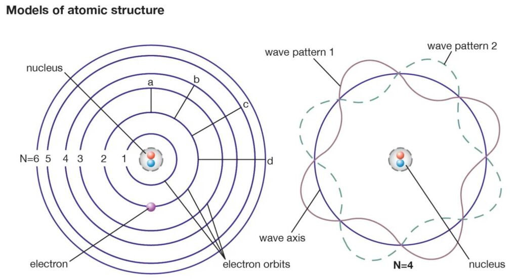
Bohr's second postulate (Hydrogen Spectrum)

i.e. 2πa = nλ …………………….(24)

where λ = h/mv

∴ 2πamv = nh or 2πamωa = nh

or ma²ω = nh / 2π

or Iω = nh / 2π (This is the same as eqn. (16))

3. Bohr’s third postulate

In order to explain how an atom emits or absorbs radiation, Bohr, following Planck’s quantum theory, made another postulate which may be stated in the following manner.

If an electron is rotating in a stationary orbit around the nucleus, for which the energy is W_i then it can shift to another stationary orbit of lower energy W_f and in doing so it will radiate energy of frequency 𝜈 given by

h𝜈 = W_i – W_f = T_f – T_i ………….(25)

Substituting the value of W from eqn. (23) or of T from eqn. (22) and giving n the values n_i and n_f corresponding to the initial and final energy states W_i and W_f respectively we get

$.\;\;\;\;\;\;\;\;\;\;\;\;\;\;\;\;\;\;\;h\nu\;=\;\frac{me^4Z^2}{8\varepsilon_o^2h^2}\left(\frac1{n_f^2}-\frac1{n_i^2}\right)$ ……………(26)

In C.G.S. unit, $h\nu\;=\;\frac{2\pi^2me^4Z^2}{h^2}\left(\frac1{n_f^2}-\frac1{n_i^2}\right)$

This equation can be written in terms of the wave number $\overline\nu$ i.e., the number of waves per meter,

$.\;\;\;\;\;\;\;\;\;\;\;\;\;\;\;\;\;\;\overline\nu\;=\frac1\lambda=\frac\nu c$

$\therefore\;\;\;\;\;\;\;\;\;\;\;\;\;\;\;\;\;\;\;\overline\nu\;=\;\frac{me^4Z^2}{8\varepsilon_o^2ch^3}\left(\frac1{n_f^2}-\frac1{n_i^2}\right)$ …………(27)

$or\;\;\;\;\;\;\;\;\;\;\;\;\;\;\;\;\;\;\;\overline\nu\;=\;RZ^2\left(\frac1{n_f^2}-\frac1{n_i^2}\right)$ …………(28)

where $R\;=\;\frac{me^4}{8\varepsilon_o^2ch^3}$ as mentioned above and is equal to 1.09678 x10⁷ /m.

For hydrogen Z = 1, therefore

$.\;\;\;\;\;\;\;\;\;\;\;\;\overline\nu=R\left(\frac1{n_f^2}-\frac1{n_i^2}\right)$ …………(29)

This is identical with the Balmer’s experimental formula for the hydrogen series (eqn.2).

Radius of Bohr’s circular orbits and the speed of orbital electrons

1. Radius of the orbits

From eqns. (13) and (22) we have

$.\;\;\;\;\;\;\;\;\;\;\;\;\;\;\frac{e^2Z}{8\pi\varepsilon_oa}=\frac{me^4Z^2}{8\varepsilon_o^2n^2h^2}$

which gives the radius of the circular orbits,

$.\;\;\;\;\;\;\;\;\;\;\;\;\;\;a=\frac{\varepsilon_oh^2}{\pi me^2}\frac{n^2}Z$ …………..(30)

This equation shows that the radius of the orbit is directly proportional to the principal quantum number n and is inversely proportional to the atomic number Z. Substituting the values of ε_o, h, m and e we get

a = 0.535 x10^-10 n²/ Z …………..(31)

For hydrogen Z = 1 and for the first orbit, n = 1; the radius for the first Bohr orbit of hydrogen therefore is

$.\;\;\;\;\;\;\;\;\;\;\;\;\;\;\;\;\;\;a_1=\frac{\varepsilon_oh^2}{\pi me^2}=0.535\times10^{-10}m$ ………….(32)

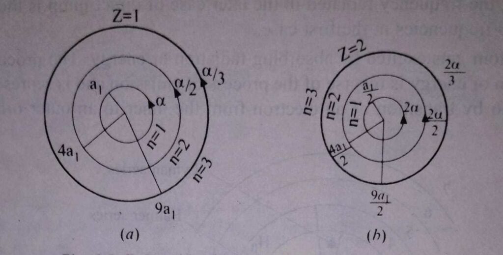
The diameter of the hydrogen atom in the normal state n = 1 therefore is about 1 A. This value is in good agreement with the value determined from collision experiments. The first three orbits of the hydrogen, Z = 1, are shown in Fig. (a) and those for ionised helium (H e⁺), Z = 2 are shown in Fig.(b) drawn to the same scale.

Bohr orbits for hydrogen and ionised helium

2. Speed of the electron in its orbit

The speed of the electron in its orbit is determined directly from eqns. (12) and (30).

$.\;\;\;\;\;\nu^2=\frac{Ze^2}{4\pi\varepsilon_oma}=\frac{Ze^2}{4\pi\varepsilon_om}\frac{\pi me^2Z}{\varepsilon_on^2h^2}$

$or\;\;\;\;\;\;\;\;\;\;\;\;\;\;\;\nu=\frac{e^2}{2\varepsilon_oh}\frac Zn$ …………(33)

The speed of the electron is therefore directly proportional to the atomic number Z and is inversely proportional to the principal quantum number n for the particular orbit. The speed of the electron as compared to the velocity of light c is given by

$or\;\;\;\;\;\;\;\;\;\;\;\;\;\;\;\frac\nu c=\frac{e^2}{2\varepsilon_och}\frac Zn$ ……….(34)

For the first Bohr orbit of hydrogen,

$or\;\;\;\;\;\;\;\;\;\;\;\;\;\;\;\frac\nu c=\alpha=\frac{e^2}{2\varepsilon_och}$ …………(35)

The constant alpha is the Sommerfeld’s fine structure constant and is important in the study of the fine structure of hydrogen series as we shall see later.

The values of α for different orbits are indicated in Fig. given above.

Bohr’s orbits and different series of hydrogen spectrum

Giving different values to n_i and n_f the different series observed in hydrogen spectrum can be calculated from eqn. (29). The transition of an electron from any of the excited states corresponding to n = 2, 3, 4….. to the first Bohr orbit, n = 1, results in the emission of a spectral line belonging to Lyman series lying in the ultra-violet region (see Fig. given below).

The transition of an electron similarly from any of the excited states n = 3, 4, 5 to the second Bohr orbit of energy state, n = 2 occurs with the emission of a spectral line belonging to Balmer series. Similar transitions give rise to spectral lines of other series as shown in Fig.

When an electron is in the third Bohr orbit, say, it may cross over to the normal state (n = 1) either by jumping first to the second orbit n = 2 and then from there to normal state n = 1 with the emission of H_α and the first line of the Lyman series, or by directly jumping to the normal state from the third orbit with the emission of a single line, the second member of the Lyman series. However as in either of the two processes the total energy radiated is the same, being equal to the difference between the energies in the third and first orbit, the frequency radiated in the later case of direct jump is the sum of the two frequencies in the first case.

An atom gets excited by absorbing radiation or energy. The process of absorption of energy is reverse of the process of emission and is represented in Fig. given above by transition of an electron from the inner to an outer orbit of larger n.

Series of ionised helium (He⁺)

It has been mentioned carlier that the Pickering series first observed in the spectrum of the star ξ-Puppis has been attributed to the ionised helium. This series can be very accurately represented by eqn.(28) because on losing one electron in ionisation He atom becomes hydrogen-like. As in the case of helium Z = 2 the Bohr’s formula for helium becomes,

$.\;\;\;\;\;\;\;\;\;\;\;\;\;\;\overline\nu=4R\left(\frac1{n_f^2}-\frac1{n_i^2}\right)$ ………….(36)

This formula, with different values of n_f and n_i represents all the known series of ionised helium. For example when n_f = 4, n_i = 5, 6, 7,…. we obtain Pickering series. The so-called λ – 4686 series of Fowler is represented by n_f = 3 and n_i = 4, 5, 6,….. Two more series which are accurately given by n_f = 2, n_i = 3, 4, 5,….. and n_f = 1, n_i = 2, 3,…… respectively have been found by Lyman in the ultra-violet region of the ionised helium spectrum.

Energy level diagram

We have seen above that energy states of the atom can be represented by orbits of increasing radii and the transitions between these states, giving rise to spectral lines, can be shown by arrows.

However when n becomes relatively large, it is rather not possible to draw orbits corresponding to these large values of n and higher series members and series limits cannot be shown on such a diagram. An energy level diagram (Fig. given below) is therefore often drawn as it is then possible to incorporate these features in the same picture. In such a diagram, each Bohr orbit or stationary state is denoted by a horizontal line drawn to an energy scale. The quantity W/hc = – R / n² which is proportional to the energy W, is usually drawn instead of plotting the energy directly. The frequency of the radiation in wave numbers $\overline\nu$ emitted as a result of a transition, is then directly given by the difference between two energy levels, for

$.\;\;\;\;\;\;\;\;\overline\nu=\frac1\lambda=\frac\nu c=\frac{W_i-W_f}{hc}$

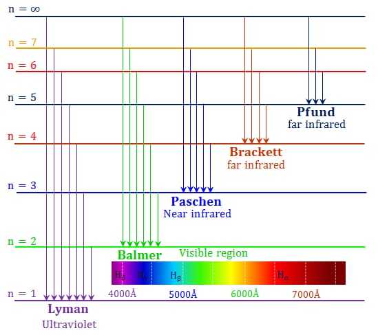
As the energy W of the quantised states have negative values and approach zero as n approaches infinity, the zero energy level corresponding to n = ∞ is drawn at the top and other energy levels are drawn below it. The energy level diagram for hydrogen is shown in Fig.given above. The arrows connecting different levels represent the transition between the corresponding energy states. Few lines of each series have also been indicated in the diagram. The energy level diagram for ionised helium can also be drawn in the same way.

Also Read :

To Wikipedia : Click Here

Hydrogen Spectrum : Lines, Series and Everything

Line and Band Spectra

Shaded Bands to Fraunhofer Lines

Equations for Balmer series